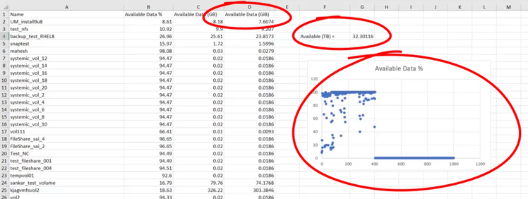
In Active IQ Unified Manager 9.8, you can bring your own excel sheets with customized reports. With this feature, you can customize existing UM reports by creating a formula, charts, etc, and upload it back into UM. Now each time the report is created manually or through a schedule, the customized report will be generated with the latest updated values. You can use this feature in 3 simple steps.
In this blog, we will walk you through how to bring in your own Excel for custom reporting.
Bring Your Own Customized Excel.
Create the view and Download the Report in Excel
- The first step would be to create a report view and save the view. In this example, we will choose the Volume inventory pages and select the required columns in the pane in Active IQ Unified Manager. After choosing the required columns, click on the “Save” icon in the “View” field and save the view.
- After you have the view saved, you can download it in Excel Workbook format (.xlsx).
Open the default, custom, or saved view that you want to use as the basis of your report. Download the report by selecting “Download Excel” under “Reports”. Save the file. The file will be saved to your downloads folder(Figure 1).

Figure 1: Download Excel Sheet

Figure 2: Customization of Excel Report
Customize the downloaded Excel Report
- Open the saved file in Excel.
- Now let’s go ahead and customize the Excel sheet report using Excel features, such as formulas, complex sorts, layered filters, or charts. Please note that you can add the sheets to the Excel file, but should not change or rename the existing “data” and the “info” sheets in the downloaded excel report.
- Now let's go ahead and customize the downloaded sheet. Create a new sheet called sample. Add the following columns on the new sample sheet:
- “Available Data %”
- “Available Data (GBs)”
- Enter the formula to sum the “Available Data and create a formula to create “Available Data (GiBs)” in Gibibytes. Make sure that it references the data sheet (data!), and references the correct column and row specifiers for the data captured .
- =SUM(data!H$2:data!H$50)
- =data!I2:data!I50*0.93
- On the data sheet, select the “Available Data %” column.Select Recommended Charts from the Insert menu and select the Scatter charts.
- Using the Design and Format menus, available when the chart is selected, you can customize how the chart looks. Save the file with your changes. Do not change the file name or location (figure 2)

Figure 3: Upload Excel
- Once the excel sheet is customized according to your preference, save the file and upload the customized the excel by selecting the Reports > Upload Excel and select the file that you modified. Make sure to upload the Excel workbook in the same view from which the report was created.
- If a customized Excel file exists, there will be a checkmark beside the Reports > Upload Excel menu item. If you upload a new customized excel workbook, it will override the existing workbook(figure 3).
- Now when you create a report with the same view or when scheduling a report, an Excel report with the customizations will be generated but updated with the latest values.
Try it Out!
We hope that you now have an idea of how to generate reports using customized Excel workbook. Try it out and do let us know your feedback. We know that you may have questions as we couldn’t cover the entire topic so please connect with us and talk to us.